A Two-Phase Dynamic Contagion Model for COVID-19
Zezhun Chen
London School of Economics Angelos Dassios
London School of Economics Valerie Kuan
University College London Jia Wei Lim
Brunel University London Yan Qu*
University of Warwick Budhi Surya
Victoria University of Wellington Hongbiao Zhao
Shanghai University of Finance and Economics
10th June 2020
*Correspondence Email: y.qu3@lse.ac.uk
In this paper, we propose a continuous-time stochastic intensity model, namely, two-phase
dynamic contagion process (2P-DCP), for modelling the epidemic contagion of COVID-19
and investigating the lockdown effect based on the dynamic contagion model introduced by
Dassios and Zhao (2011). It allows randomness to the infectivity of individuals rather than a
constant reproduction number as assumed by standard models. Key epidemiological quantities,
such as the distribution of final epidemic size and expected epidemic duration, are derived and
estimated based on real data for various regions and countries. The associated time lag of the
effect of intervention in each country or region is estimated. Our results are consistent with
the incubation time of COVID-19 found by recent medical study. We demonstrate that our
model could potentially be a valuable tool in the modeling of COVID-19. More importantly,
the proposed model of 2P-DCP could also be used as an important tool in epidemiological
modelling as this type of contagion models with very simple structures is adequate to describe
the evolution of regional epidemic and worldwide pandemic.
Keywords: Stochastic intensity model; Stochastic epidemic model; Two-phase dynamic contagion process; COVID-19;
Lockdown
Mathematics Subject Classification (2010): Primary: 60G55; Secondary: 60J75
JEL Classification: I1; H0; E6
1 Introduction
In the early stages of epidemic modelling, the spread of diseases was formulated as a deterministic
process. The classical deterministic model of susceptible-infectious-recovered (SIR) was introduced in the
seminal paper of Kermack and McKendrick (1927). It models the spread and ultimate containment of an
infection in a setting where those who recover are immune to the disease and thus the susceptible
population declines over time. Many epidemic models are variations of the SIR model, see Brauer
et al. (2008); Keeling and Rohani (2008); Diekmann et al. (2013) and Martcheva (2015). For
example, during the outbreak of COVID-19 since December 2019, a commonly adopted approach for
predicting the number of infections is the susceptible-exposed-infectious-recovered (SEIR) model, which
adds an exposed period to the SIR model for accounting the reported incubation period of COVID-19
during which individuals are not yet infectious, e.g. Berger et al. (2020); Liu et al. (2020) and Tian
et al. (2020). More recently, Acemoglu et al. (2020) develop a multi-risk SIR model, which takes into
account that different subpopulations have different risks and is applied to analysing optimal lockdown.
However, the random nature of the epidemics spread in our real world suggests that a stochastic
model is needed. A continuous-time stochastic counterpart of SIR model was first proposed by
McKendrick (1925), and then a variety of stochastic models were studied in the literature, e.g.
Bartlett (1949, 1956) and Bailey (1950, 1953, 1957). For more recent developments on stochastic
epidemic models in general, see Daley and Gani (1999); Andersson and Britton (2000); Allen (2008)
and Fuchs (2013). In particular, many researchers adopted branching processes. Ball (1983) used the
birth-and-death process for constructing a sequence of general stochastic epidemics, and Ball and
Donnelly (1995) used branching processes to approximate the early stages of epidemic dynamics, see
also Britton (2010) and Ball et al. (2016).
In this paper, we propose a continuous-time stochastic epidemic model, namely, the two-phase
dynamic contagion process (2P-DCP), for modelling the epidemic contagion. It is a branching
process, and can be considered as a generalisation of dynamic contagion process (Dassios
and Zhao, 2011), which is an extension of the classical Hawkes process (Hawkes, 1971a,b).
In fact, Hawkes process and its various generalisations were originally used for modelling
earthquakes in seismology, and recently become extremely popular for modelling financial
contagion in economics, see Bowsher (2007); Large (2007); Embrechts et al. (2011); Bacry
et al. (2013a,b); Aït-Sahalia et al. (2015); Dassios and Zhao (2017a,b) and Qu et al. (2019).
Analogously, we advocate that they are also applicable to epidemiology. As not all individuals are
equally infectious in reality, the main advantage of this Hawkes-based approach is that, it allows
randomness to the infectivity of individuals, rather than a constant reproduction number (the average
number of subsequent infections of an infected individual) in standard models. In this paper, we
adopt the 2P-DCP as a more realistic and parsimonious example of Hawkes-based models
for modelling the current progression of COVID-19 and investigating the lockdown effect.
Key epidemiological quantities, such as the distribution of final epidemic size and expected
epidemic duration, have been derived and estimated based on real data. Pandemics have largely
shaped the history of human being as described in the popular book by McNeill (1976), and
have made huge impacts to our society and and economy. However, mathematical models
developed in epidemiology and economics don’t talk to each other much until the current
outbreak of COVID-19, which needs urgent calls (e.g. from The Royal Society) for researchers
across disciplines to work together and jointly support the scientific modelling for epidemics,
see recent intensive interplays between the two fields, e.g. Acemoglu et al. (2020); Alvarez
et al. (2020); Atkeson (2020); Eichenbaum et al. (2020) and Guerrieri et al. (2020). Our paper also
responds to the calls by introducing the Hawkes-based approach as a potentially very valuable tool for
epidemic modelling.
This paper is organised as follows: Section 2 offers the preliminaries including an introduction and
formal mathematical definitions for our stochastic epidemic model, a two-phase dynamic contagion
process. Key distributional properties, such as the distribution of final epidemic size and expected
epidemic duration, are provided in Section 3. In Section 4, our model is implemented based on real data,
and the associated time lag of the effect of intervention in each country or region is estimated. Finally,
Section 5 draws a conclusion for this paper, and proposes some issues for possible further extensions and
future research.
2 Two-Phase Dynamic Contagion Process
In this section, we introduce a two-phase dynamic contagion process (2P-DCP) for modelling the
dynamics of COVID-19 contagion. The unobservable effective time that aggregated government
interventions (e.g. lockdown of a city or country) came into effect is denoted by ℓ > 0, which divides the
COVID-19 epidemic dynamics into two phases. Note that, the time point ℓ is different from the exact
timing of intervention that can be observed. The cumulated number of infected individuals is described by
a counting process Nt with N0 = 0, and it is modelled by a two-phase dynamic contagion process
defined as below.
Definition 2.1 (Two-Phase Dynamic Contagion Process (2P-DCP)). A two-phase dynamic contagion
process (2P-DCP) is a point process Nt with two phases:
-
Phase 1 (Full Contagion):
- For the first phase period t ∈ [0,ℓ), Nt follows a dynamic contagion process
with stochastic intensity
![*
-δt ∑Nt -δ(t- T*) N∑t -δ(t- T)
λt = λ0e + Zke k + Yie i, t ∈ [0,ℓ],
k=1 i=1](Paper_Covid_19_DCP0x.png) | (2.1) |
where
- λ0 > 0 is the initial intensity at time t = 0;
- δ > 0 is the constant rate of exponential decay;
- Nt*≡{Tk*}k=1,... is a Poisson process of constant rate ϱ > 0 arriving in time t ≤ℓ;
- {Zk}k=1,...,Nℓ* are i.i.d. externally-exciting jump sizes, realised at times
{Tk*}k=1,...,Nℓ*, with distribution H(y);
- {Y i}i=1,...,Nℓ are i.i.d. self-exciting jump sizes of the first phase, realised at times
{Ti}i=1,...,Nℓ , with distribution G1(y).
-
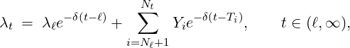
Phase 2 (Self Contagion):
- For the second phase period t ∈ (ℓ,∞), Nt is a pure self-exciting Hawkes
process with stochastic intensity
 | (2.2) |
where
- λℓ is the initial intensity of the second phase starting at the cutoff time point ℓ, which
is the terminal intensity of the first phase;
- {Y i}i=Nℓ+1,... are i.i.d. self-exciting jump sizes of the second phase, realised at times
{Ti}i=Nℓ+1,..., with distribution G2(y). Note that compared with the average mean of
the self-exciting jump size for Phase 1, the mean of self-exciting jump in Phase 2 is
smaller, which demonstrates that the COVID-19 becomes less contagious on average
after time point ℓ.
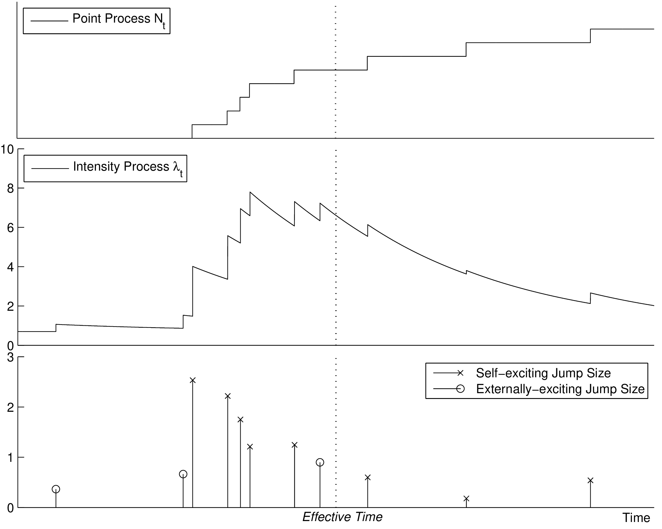
The point process Nt and its intensity process λt are illustrated in Figure 1. Overall, we can more
compactly define our new pandemic model, a two-phase dynamic contagion process, as a counting
process Nt ≡{Ti}i=1,... with N0 = 0 and stochastic intensity
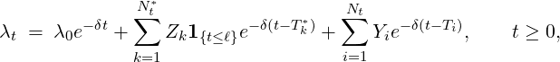 | (2.3) |
where
- {Y i}i=1,...Nt are i.i.d. self-exciting jump sizes with a two-phase distribution G(y;t),
i.e.,
 | (2.4) |
- {Zk}k=1,...Nt* are i.i.d. externally-exciting jump sizes with distribution H(y).
This equivalent definition as a dynamic contagion process has an advantage: it can be viewed as a
branching process and has a more intuitive interpretation with regard to a pandemic. The cluster-process
presentation is provided as follows.
- The cumulated number of infected cases, Nt, is a cluster point process, which consists of
two types of points: outside-imported cases and inside-infected cases.
- The arrivals of outside-imported cases follows a Cox process with shot-noise intensity
|
λ0e-δt + ∑
k=1Nt*
Zke-δ(t-Tk*),
|
where externally-exciting jumps arrive as a Poisson process Nt* at time points {Tk*}k=1,...
with sizes (marks) {Zk}k=1,..., and they disappear after time point ℓ when the interventions
took effect, and there will be no any increase of imported cases in a long run.
- Each imported case may infect other individuals inside and thereby causes new cases, and
each of these new cases would further infect others inside, and so on. The infection of any
new cases caused by the previous infected cases follows a Cox process with exponentially
decaying intensity Y ⋅e-δ(t-T⋅), where Y ⋅ follows a two-phase distribution G(y;t) and T⋅
is the infection time of the previous infected case. After the interventions took effect, the
COVID-19 becomes less easy to spread on average. This is captured by our assumption of
two-phase distribution (2.4) for Y ⋅ here.
- Overall, the superposition of all these infected cases form a point process Nt, a two-phase
dynamic contagion process with stochastic intensity (2.3).
3 Distributional Properties
In this section, we outline key distributional properties for the two-phase dynamic contagion process. We
derived the conditional joint Laplace transform of λt and probability generating function of Nt, which are
the key results to further derive the elimination probability of the epidemic and the distribution of the final
epidemic size.
Joint Distribution of (λt,Nt)
Let { t}t≥0 be the natural filtration of the point process Nt, i.e. t = σ
 and assume that the
intensity process {λt}t≥0 being t-adapted. The joint Laplace transform and probability generating
function for (λt,Nt) is provided in Theorem 3.1 as below.
and assume that the
intensity process {λt}t≥0 being t-adapted. The joint Laplace transform and probability generating
function for (λt,Nt) is provided in Theorem 3.1 as below.
Theorem 3.1. For time s ≤t, the conditional joint Laplace transform and probability generating
function for λt and the point process Nt is of the form
where A(s) is determined by the nonlinear ordinary differential equation (ODE)
 | (3.2) |
where the boundary condition is A(t) = v with
|
ĝ(u;t) = ∫
0∞e-uydG(y;t),
|
and c(t) is determined by
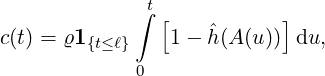 | (3.3) |
with
Proof. For 0 ≤s ≤t ≤ℓ, λt is the intensity process of the dynamic contagion process introduced in
Dassios and Zhao (2011). The corresponding conditional joint Laplace transform, probability
generating function for the process λt and the point process Nt is provided in Theorem 3.1 of
Dassios and Zhao (2011). For ℓ < s ≤t, given s, the infinitesimal generator of the dynamic
contagion process (λs,Ns,s) acting on a function f(λ,n,s) within its domain Ω( ) is given
by
) is given
by
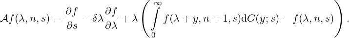 | (3.4) |
Consider a function f(λ,n,s) of form
and substitute this into f = 0, we then have the ODE
A′(s) = δA(s) - 1 + θĝ A(s),s A(s),s , ,
|
adding the boundary condition A(t) = v, gives the ODE in (3.2). __
The moments of λt and Nt can be obtained by differentiating the joint Laplace transform and
probability generating function of λt and Nt, and the results are provided in Proposition 3.1 and 3.2 as
below.
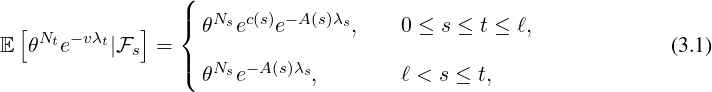
Proposition 3.1. The conditional expectation of the process λt given s for s ≤t is given by
and the conditional expectation of the point process Nt given s is of the form where
|
μH = ∫
0∞ydH(y), μ
G = ∫
0∞ydG
1(y)1{t≤ℓ} + ∫
0∞ydG
2(y)1{t>ℓ},
|
and κ = δ -μG.
Proof. The result in (3.5) immediately follows Theorem 3.6 in Dassios and Zhao (2011). And since
Nt -Ns -∫
stλ
udu is a martingale, we have
E![[Nt - Ns |Fs]](Paper_Covid_19_DCP13x.png) = ∫
stE = ∫
stE![[λu|Fs ]](Paper_Covid_19_DCP14x.png) du, du,
|
which directly implies the result in (3.6). __
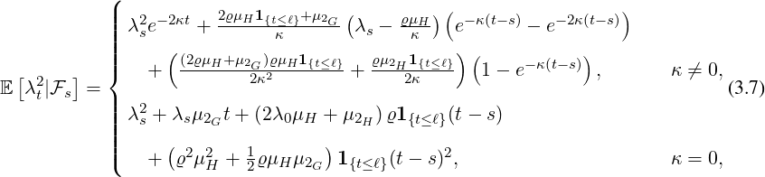
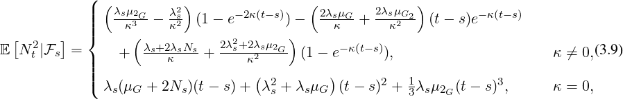
Proposition 3.2. The conditional second moment of the process λt given s for s ≤t is given by
and the conditional joint expectation of the process λt and the point process Nt given s for s > ℓ is of
the form and the second moment of point process Nt given s for s > ℓ is of the form where
|
μ2H = ∫
0∞y2dH(y), μ
2G = ∫
0∞y2dG
1(y)1{t≤ℓ} + ∫
0∞y2dG
2(y)1{t>ℓ},
|
and κ = δ -μG.
Proof. These results immediately follows Lemma 3.1, Lemma 3.2 and Theorem 3.9 in Dassios and
Zhao (2011). __
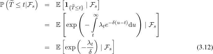
Probability of Elimination Time 
After the government interventions come into effect, the contagion rate will dramatically decline
and new cases will drop abruptly almost to nothing in the near future. It is therefore of great
interests to calculate the probability of elimination time, i.e. the time that the last ever case
arrives, after government interventions come into effect. Let  to be elimination time such
that
to be elimination time such
that
 | (3.10) |
The condition probability of the elimination time is provided in Proposition 3.3.
Proposition 3.3. For ℓ ≤s ≤t, the elimination probability is given by
 | (3.11) |
where A(s) is determined by the ODE in (3.2) with boundary condition A(t) =  .
.
Proof. Given  being the timing of the last ever event, the event {
 ≤t} implies that Nu = Nt for any
u ≥t, which also lead to
≤t} implies that Nu = Nt for any
u ≥t, which also lead to
Hence, we have
And according to Theorem
3.1, by setting
θ = 1 in (
3.1), the result follows immediately. __
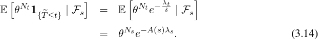
Joint Expectation of Epidemic Size Nt and Elimination Time 
Given the last ever event { < t}, one could obtain the expected size of the epidemic at time t. The
relevant details are presented in Corollary 3.1.
< t}, one could obtain the expected size of the epidemic at time t. The
relevant details are presented in Corollary 3.1.
Corollary 3.1. For ℓ ≤s ≤ ≤t, the conditional joint expectation of Nt and 1{
 ≤t}is of the following
form
≤t}is of the following
form
where A(s) satisfies the ODE in (
3.2)
with boundary condition A(t) =  .
.
Proof. According to Theorem 3.1 and Proposition 3.3, we have
Since
E =
=  E
E
 θ=1-
θ=1-
, the result immediately follows
(
3.13).
__
Distribution of Final Epidemic Size N∞
The final epidemic size is one of the most important epidemiological quantities to study. In
fact, under the two-phase dynamic contagion model, the final epidemic size is the value of
the point process Nt when time goes to infinity. Conditional on s > ℓ, since there are no
externally-exciting jumps in the intensity, the distribution of N∞ can be characterised by Proposition 3.4
as below.
Proposition 3.4. For ℓ < s, the probability generating function of N∞conditional on s is given
as
 | (3.15) |
where
v* =   . .
|
While the government interventions come into effect, if we assume i.i.d. self-exciting jump sizes
Y i ~ Exp(β) for i = Nℓ + 1,...., then, we have an explicit expression for the probability generating
function of N∞ as
E[θN∞
∣s] = exp , s > ℓ. , s > ℓ.
|
This implies that, the final epidemic size N∞ conditional on ℓ follows a mixed-Poisson distribution with
the probability mass function
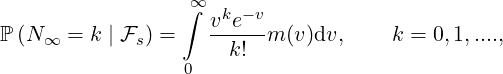 | (3.16) |
where m(v) is the density function of the mixing distribution,
m(v) := exp  , ,
|
which is an inverse Gaussian distribution with parameters  λs and
  λs2.
λs2.
4 Empirical Study
We provide a calibration scheme based on the daily increments of the two-phase dynamic contagion
process Nt. Let us first denote the observations of the daily confirmed COVID-19 cases as
{Ct}t=0,1,2,...,T . The mean square error (MSE) between the expected daily increments of Nt and the
actual reported daily confirmed COVID-19 cases is given as
![T-1
1-∑ 2
MSE (α,β,δ,ϱ,ℓ) = T (E [Nt+1 - Nt ]- Ct+1) .
t=0](Paper_Covid_19_DCP46x.png) | (4.1) |
We consider the calibration based on minimising the MSE (4.1), i.e., we choose parameters ( ,
, ,
, ,
, ,
, )
such that
)
such that
MSE( , , , , , , , , ) := min(α,β,δ,ϱ,ℓ)MSE(α,β,δ,ϱ,ℓ), ) := min(α,β,δ,ϱ,ℓ)MSE(α,β,δ,ϱ,ℓ),
|
with α,β,δ,ϱ ≥ 0 and ℓ ∈ℕ+.
Without loss of generality, for simplicity, we assume Zk = 1 for any k, Y i ~ Exp(α) for i = 1,...,Nℓ
and Y i ~ Exp(β) for i = Nℓ + 1,..., and λ0 = 0 in (2.3) for model calibration. Other assumptions for
Zk,{Y i}i=1,...Nℓ,Nℓ+1,...,λ0 can also be used if necessary. We provide two empirical examples. The first
one concentrates on the COVID-19 pandemic in mainland China during the period from early January to
late March 2020. The second one focuses on the worldwide COVID-19 pandemic during
the period from mid February to early May 2020. The data we used are publicly available.
Datasets are mostly cited from the associated official government health department websites for
non-European countries and from the European Centre of Disease Control (ECDC) for European
countries.
COVID-19 Pandemic in Mainland China
The daily confirmed COVID-19 cases for regions in China can be obtained from daily reports of the
National Health Commission of the PRC. We use the reported daily confirmed cases for several
regions in China from 2020-01-19 to 2020-03-31 as examples for model calibration. The
corresponding estimation results are illustrated in Table 1. We can see that the estimator  are quite
different from each other. In particular, these regions that are close to Hubei, namely Henan,
Hunan, Anhui, have relatively larger intensities for externally-exciting jumps, which means
that these regions experienced more external shocks from Wuhan and these external shocks
can be originally infected individuals from Wuhan. Naturally, without taking into account
Wuhan, the rest of Hubei has the largest intensity
are quite
different from each other. In particular, these regions that are close to Hubei, namely Henan,
Hunan, Anhui, have relatively larger intensities for externally-exciting jumps, which means
that these regions experienced more external shocks from Wuhan and these external shocks
can be originally infected individuals from Wuhan. Naturally, without taking into account
Wuhan, the rest of Hubei has the largest intensity  for externally-exciting jumps. The main
government intervention established by the Chinese authority is the announcement of the
completely lockdown of Wuhan and later the whole Hubei Province on 23 January 2020.
One or two days later, all other regions enforced the quarantine and raised the alert of public
health emergency. Setting the date 2020-01-19 as the initial time t = 0, then the government
intervention took place when t = 4 and came into effect when t =
for externally-exciting jumps. The main
government intervention established by the Chinese authority is the announcement of the
completely lockdown of Wuhan and later the whole Hubei Province on 23 January 2020.
One or two days later, all other regions enforced the quarantine and raised the alert of public
health emergency. Setting the date 2020-01-19 as the initial time t = 0, then the government
intervention took place when t = 4 and came into effect when t =  . Since the delay period of the
government interventions is the difference of the date when the government interventions came
into effect and the date when the government introduced the restriction measures, we can
therefore observe from Table 1 that the estimated delays of the government interventions for
different regions therefore are between 5 and 15 days, which are consistent to the incubation
time of COVID-19 for most people, e.g. as found in a highly cited medical study of Lauer
et al. (2020).
. Since the delay period of the
government interventions is the difference of the date when the government interventions came
into effect and the date when the government introduced the restriction measures, we can
therefore observe from Table 1 that the estimated delays of the government interventions for
different regions therefore are between 5 and 15 days, which are consistent to the incubation
time of COVID-19 for most people, e.g. as found in a highly cited medical study of Lauer
et al. (2020).
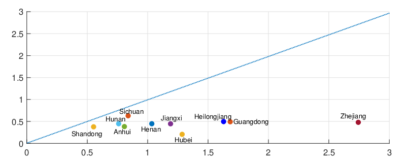
The branching ratio (BR), which demonstrates the average infection rate, is determined by E[Y i]∕δ.
In Table 2, we compare the estimated branching ratios before and after the government interventions came
into effect, namely Rb and Ra, respectively. It is clear that the branching ratio for every region decreases
significantly when the state changed, i.e. government interventions came into effect. One can also access
the efficiency for when regions implemented the restriction packages introduced by the central
government by comparing the corresponding branching ratios Rb and Ra. The comparison of
Rb and Ra for regions in China are presented in Figure 2. We can see that the government
restriction packages had been well-implemented for all regions in China. In particular, Hubei,
where the strictest measure, i.e. the completely lockdown of Wuhan and Hubei, had been
introduced, shows a dramatic drop of contagion rate after the interventions came into effect.
Table 2: The estimated branching ratio (BR) before and after the government interventions came
into effect, namely Rb,Ra respectively, for regions in China.
_________________________________________________________________
|
|
|
 | Rb | Ra |
|
|
|
|
|
|
| Heilongjiang | 1.630176 | 0.493166 |
|
|
|
| Sicuan | 0.840021 | 0.625153 |
|
|
|
| Shandong | 0.554130 | 0.373512 |
|
|
|
| Jiangxi | 1.191025 | 0.442510 |
|
|
|
| Anhui | 0.809039 | 0.379250 |
|
|
|
| Hunan | 0.761641 | 0.444234 |
|
|
|
| Zhejiang | 2.744989 | 0.476066 |
|
|
|
| Henan | 1.035957 | 0.443853 |
|
|
|
| Guangdong | 1.685052 | 0.488747 |
|
|
|
| Hubei | 1.287094 | 0.202028 |
|
|
|
| |
_________________________________________________________________
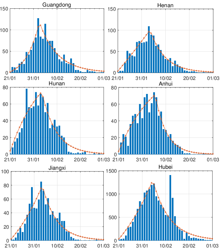
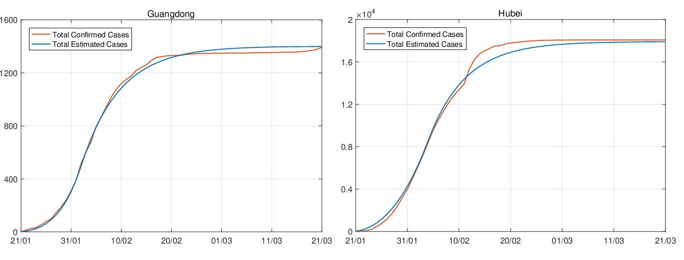
Figure 3 and 4 demonstrate comparisons between the expected daily/total confirmed cases for the
two-phase dynamic contagion model under the calibrated parameter ( ,
, ,
, ,
, ,
, ) in Table 1 and the
actual daily/total confirmed COVID-19 cases for the period 2020-01-19 to 2020-03-31. We observe that
the model allows different shapes of trend before the interventions came into effect. All these regions
indicate relatively smooth exponential decay of daily new cases after the peak. In addition, the estimated
cumulative confirmed cases are very close to the actual total confirmed COVID-19 cases,
which further confirms that our new model is a good candidate for describing the propagation
process.
) in Table 1 and the
actual daily/total confirmed COVID-19 cases for the period 2020-01-19 to 2020-03-31. We observe that
the model allows different shapes of trend before the interventions came into effect. All these regions
indicate relatively smooth exponential decay of daily new cases after the peak. In addition, the estimated
cumulative confirmed cases are very close to the actual total confirmed COVID-19 cases,
which further confirms that our new model is a good candidate for describing the propagation
process.
COVID-19 Pandemic for the World
From mid-February 2020, the COVID-19 started to spread in other countries around the world. At
beginning, only a small number of initial cases were reported for some countries in Europe, South/East
Asia and North American. However, lately, several large outbreaks were reported in South
Korea, Italy, Iran, Spain, Japan and the total number of cases outside China quickly passed the
China’s. The WHO then recognized the spread of COVID-19 as pandemic on 2020-03-11. We
could use this as a second example to confirm our observations from the last exercise. The
calibration settings were the same as the previous one. We use the reported daily confirm cases for
different regions and countries around world from mid-February to early May 2020. Note that,
due to the fact that the pandemic reached each country or territory at different time and the
corresponding government interventions also imposed and came into effect at different times,
there is no sense to calibrate the model using the data within the same truncated time series.
Table 3 presents the estimation results ( ,
, ,
, ,
, ,
, ) of (α,β,δ,ϱ,ℓ) for various countries
and territories. We notice that regions and countries like Italy, China, New York have much
larger ϱ compared with other areas. This phenomena is reasonable as these areas have specific
outbreak area which created external shocks to other part of the regions and countries and
hence the number of confirmed cases increased more rapidly than other regions and countries.
) of (α,β,δ,ϱ,ℓ) for various countries
and territories. We notice that regions and countries like Italy, China, New York have much
larger ϱ compared with other areas. This phenomena is reasonable as these areas have specific
outbreak area which created external shocks to other part of the regions and countries and
hence the number of confirmed cases increased more rapidly than other regions and countries.
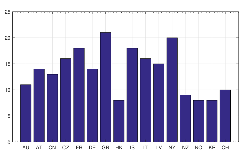
In Table 3, we also presents the date of day 0, i.e. Date0, and the date of government interventions
imposed, i.e. DateG. The delay period of government interventions came into effect therefore can be
obtained given the estimated  , with Date0 and DateG. The details for the delay periods of regions and
countries are illustrated in Figure 5. We can see that the delay of the interventions for different
regions and countries is around 8 ~ 21 days. In fact, the delay period can be considered as a
criteria for evaluating the effectiveness of restrictions imposed by the authorities to prevent
further spread of COVID-19. In general, most regions and countries with short delay periods
normally took tougher restrictions or more effective measures to stop the spread of virus. New
Zealand and South Korea are two typical examples. The authority of New Zealand introduced a
nationwide lockdown by closing all borders and entry ports to all nonresidents. On contrary,
the South Korea authority introduced one of the largest and best-organised epidemic control
programs to screen the mass population for the virus with isolation, tracing, quarantine took place
simultaneously without further lockdown. Therefore, the estimated delay periods for these
two countries are only 9 days for New Zealand and 8 days for South Korea, which are much
shorter than the average incubation time of COVID-19. For most European countries, due to the
containment restriction measures such as quarantines and curfews were not strictly put into
effect, the associated delay periods are relatively longer than the incubation time of COVID-19.
, with Date0 and DateG. The details for the delay periods of regions and
countries are illustrated in Figure 5. We can see that the delay of the interventions for different
regions and countries is around 8 ~ 21 days. In fact, the delay period can be considered as a
criteria for evaluating the effectiveness of restrictions imposed by the authorities to prevent
further spread of COVID-19. In general, most regions and countries with short delay periods
normally took tougher restrictions or more effective measures to stop the spread of virus. New
Zealand and South Korea are two typical examples. The authority of New Zealand introduced a
nationwide lockdown by closing all borders and entry ports to all nonresidents. On contrary,
the South Korea authority introduced one of the largest and best-organised epidemic control
programs to screen the mass population for the virus with isolation, tracing, quarantine took place
simultaneously without further lockdown. Therefore, the estimated delay periods for these
two countries are only 9 days for New Zealand and 8 days for South Korea, which are much
shorter than the average incubation time of COVID-19. For most European countries, due to the
containment restriction measures such as quarantines and curfews were not strictly put into
effect, the associated delay periods are relatively longer than the incubation time of COVID-19.
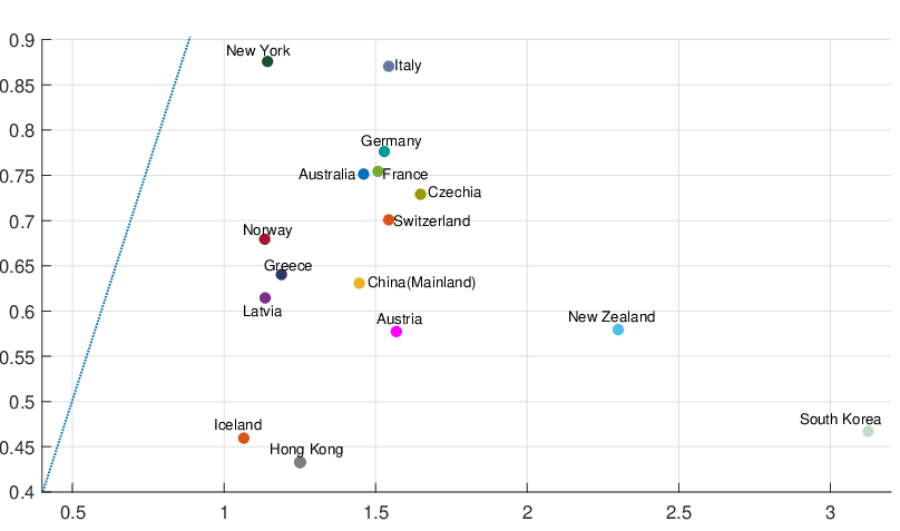
The estimated branching ratios before and after the government interventions came into effect for
different countries and territories are reported in Table 4. And Figure 6 demonstrates a comparison
between the BRs before the government interventions took effect and the BRs after the interventions
worked, with a blue dash line that represents Rb = Ra. We can immediately see that for most regions and
countries, the BR dropped dramatically after government interventions came into effect, which suggests
that the restriction measures imposed by the authority indeed reduce the contagion/infection rate
significantly.
Table 4: The estimated branching ratio (BR) before and after the government interventions came
into effect, namely Rb,Ra respectively, for regions and countries around the would.
_________________________________________________
|
|
|
 | Rb | Ra |
|
|
|
|
|
|
| Australia | 1.461638 | 0.750991 |
|
|
|
| Austria | 1.569681 | 0.576945 |
|
|
|
| China(Mainland) | 1.447200 | 0.630380 |
|
|
|
| Czechia | 1.649399 | 0.728637 |
|
|
|
| France | 1.509016 | 0.753908 |
|
|
|
| Germany | 1.529826 | 0.775845 |
|
|
|
| Greece | 1.190377 | 0.639993 |
|
|
|
| Hong Kong | 1.252077 | 0.432526 |
|
|
|
| Iceland | 1.066200 | 0.459162 |
|
|
|
| Italy | 1.544364 | 0.870102 |
|
|
|
| Latvia | 1.136798 | 0.614084 |
|
|
|
| New York | 1.144667 | 0.875377 |
|
|
|
| New Zealand | 2.301455 | 0.579001 |
|
|
|
| Norway | 1.135488 | 0.678991 |
|
|
|
| South Korea | 3.125643 | 0.466606 |
|
|
|
| Switzerland | 1.544349 | 0.700379 |
|
|
|
|
|
|
| |
_________________________________________________
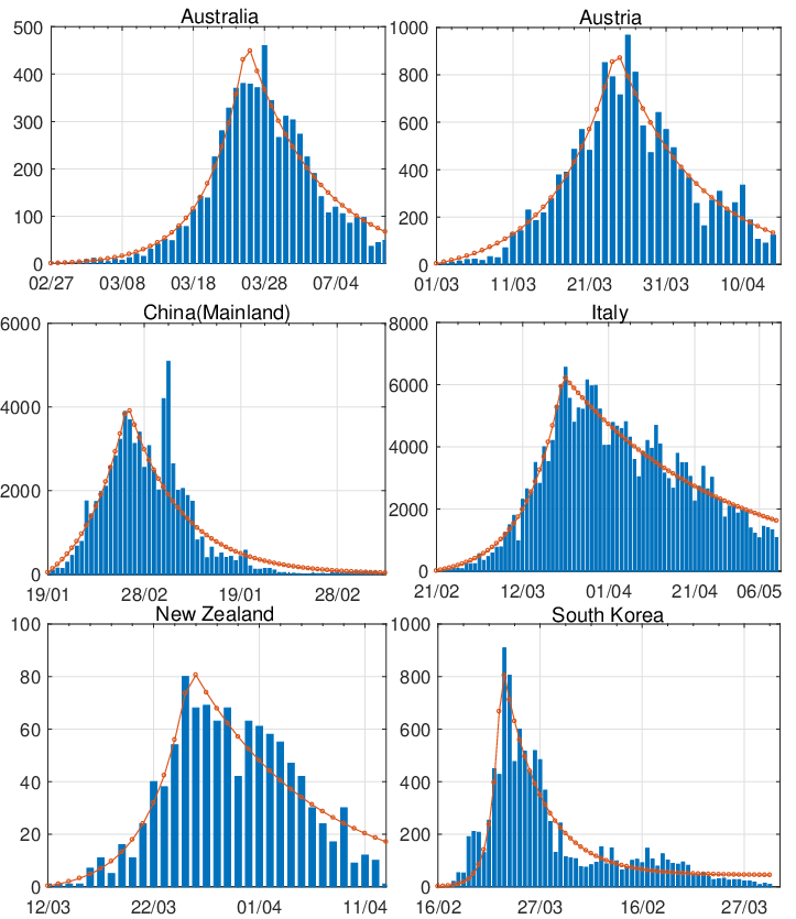
A comparison between the expected daily confirmed cases for the two-phase dynamic contagion
model under the calibrated parameters ( ,
, ,
, ,
, ,
, ) is reported in Table 3, and the actual daily confirmed
COVID-19 cases for different regions and countries over the period of mid-February to early May are
presented in Figure 7. In general, we can see that the model can precisely catch the trend of infection, this
further confirms that the two-phase dynamic contagion model is effective. Note that, we have smoothed
the biggest jump of daily confirmed cases in China for better illustration and fitting purpose.
This is due to a change in the confirmation standard established by the Chinese authority on
2020-02-12.
) is reported in Table 3, and the actual daily confirmed
COVID-19 cases for different regions and countries over the period of mid-February to early May are
presented in Figure 7. In general, we can see that the model can precisely catch the trend of infection, this
further confirms that the two-phase dynamic contagion model is effective. Note that, we have smoothed
the biggest jump of daily confirmed cases in China for better illustration and fitting purpose.
This is due to a change in the confirmation standard established by the Chinese authority on
2020-02-12.
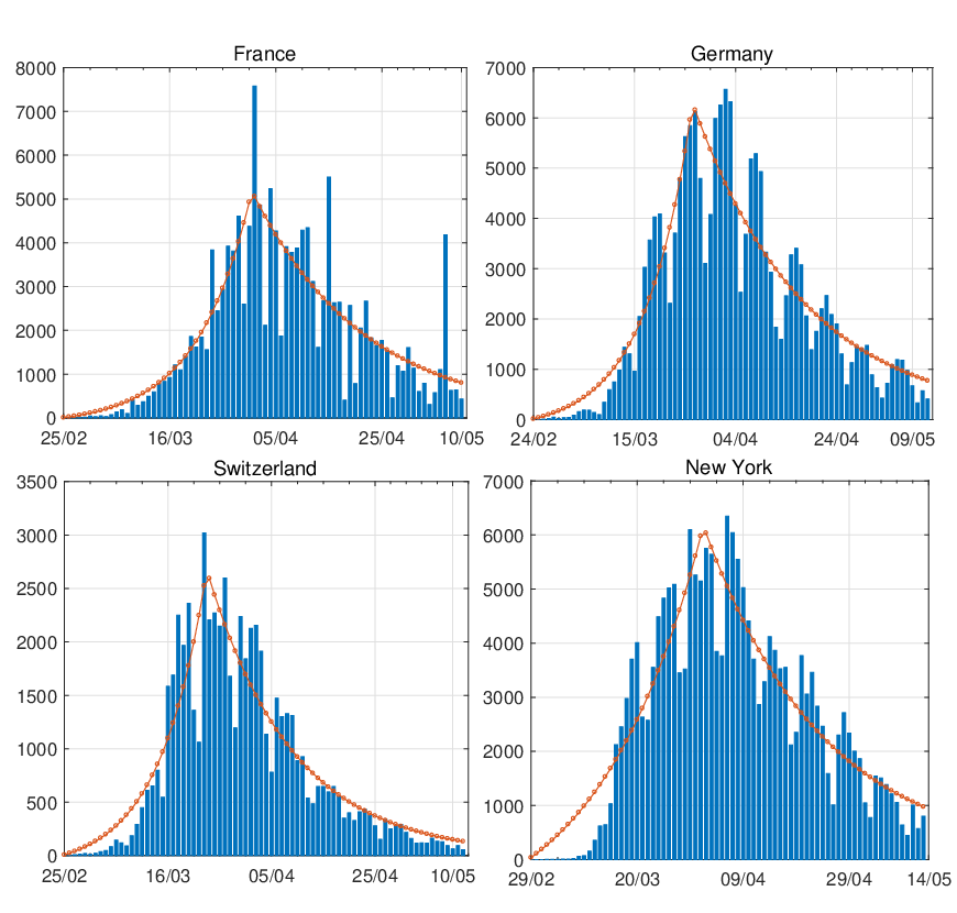
In Figure 8, we compare the estimated daily increment with the actual confirmed COVID-19 cases
for France, Germany, Switzerland, and New York. The daily records of confirmed cases for
these areas were not as smooth as those countries illustrated in Figure 7. The spikes within
the graphs could be caused by many reasons such as the delay of reports, testing capacity,
hospital capacity, diagnostic methods and etc. For instance, the daily confirmed cases for France,
Germany, Switzerland and New York suddenly declined on a regular basis, which mostly
happened during the weekends. Even so, we can see the model can still capture the trend
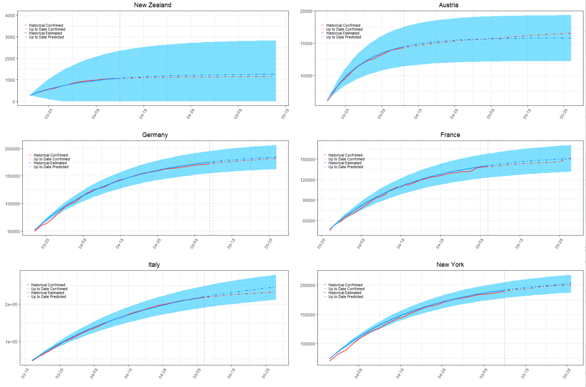
of infectious evolution. In Figure 9, we also compare the actual total confirmed COVID-19
cases against the cumulative estimated cases with a confidence interval within two standard
deviations
for some typical countries and territories. The black dash line in each graph of Figure 9 represents the end
of data collection period for calibration. The red curve on the left of the black dash line shows the
historical data used for calibration and the blue curve is the corresponding estimated result. The red and
blue curves on the right of the black dash line demonstrate a comparison between the predicted and actual
confirmed COVID-19 cases for countries and regions from the end of their data collection period to the
end of May, 2020. We can see that the estimated curves of the number of confirmed infections
under the two-phase dynamic contagion model well fitted the actual propagation process of
the COVID-19. In addition, the forecasted infection cases in the coming weeks after the end
of data collection period also well suited the up to date actual total confirmed COVID-19
cases.
4.1 Elimination Probability and Final Epidemic Size
According to Proposition 3.3, one could obtain the elimination probability of the epidemic by numerically
solving the ODE (3.2). Based on the calibration parameters ( ,
, ,
, ,
, ,
, ) provided in Table 3 for regions
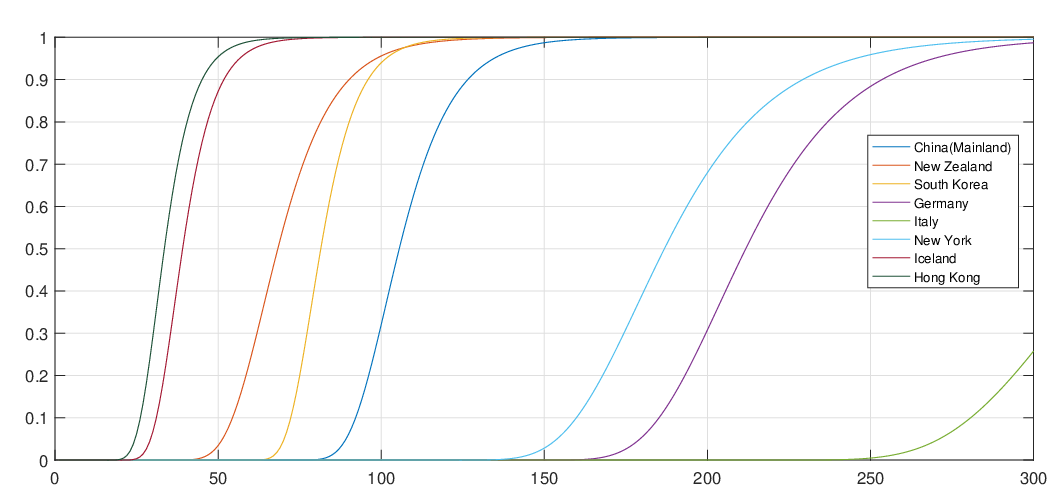
and countries, we could obtain the associated elimination probabilities. Figure 10 illustrates how
ℙ
) provided in Table 3 for regions
and countries, we could obtain the associated elimination probabilities. Figure 10 illustrates how
ℙ varies for different countries and territories. We can see that for regions and countries with
effective restriction measures, the probability for a shorter period to observe the last ever event arrives
after government interventions come into effect will be much higher. On contrary, for some regions
and countries, longer periods are needed for elimination probabilities to be closed to 1. For
instance, we can see that there is still a long way to go to end the COVID-19 pandemic for
Italy.
varies for different countries and territories. We can see that for regions and countries with
effective restriction measures, the probability for a shorter period to observe the last ever event arrives
after government interventions come into effect will be much higher. On contrary, for some regions
and countries, longer periods are needed for elimination probabilities to be closed to 1. For
instance, we can see that there is still a long way to go to end the COVID-19 pandemic for
Italy.
The elimination time of the pandemic depends on many decisive factors, such as the initial intensity of
the externally-exciting jumps, the time needed for the government interventions to come into effect, the
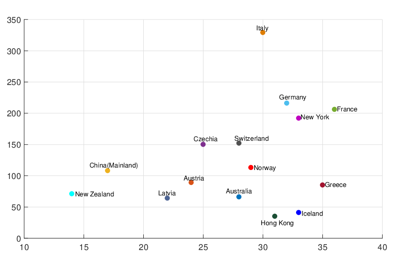
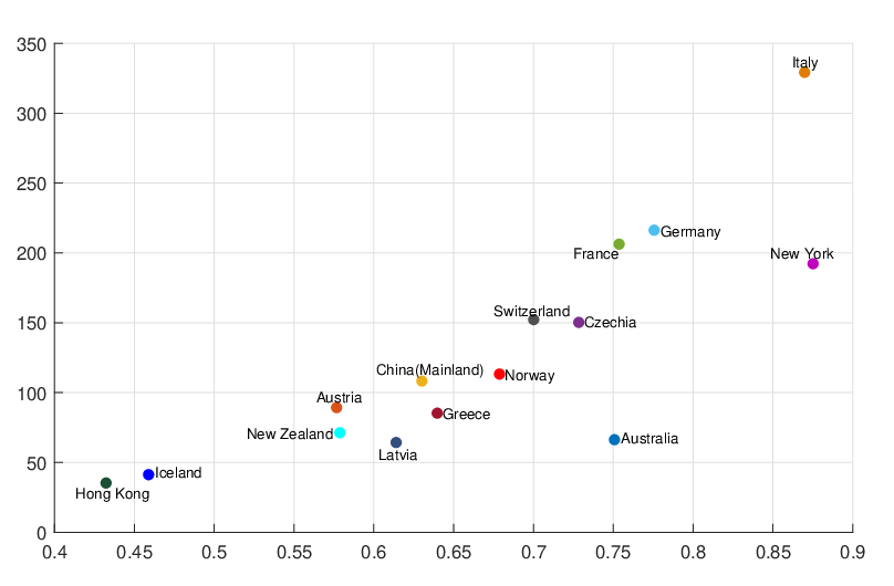
size of the branching ratio after the government interventions came into effect, etc. Figure 11, 12,
and 13 illustrate comparisons between the estimated  ,
,  , Ra against E[
 |
| ], respectively.
From Figure 11, we can see that for most countries and territories, the quicker the government
interventions come into effect, the faster the pandemic will end. However, some places like Hong
Kong and Iceland still have relatively fast elimination time even though it takes longer for
the government interventions to come into effect. This is probably because the restriction
measures for these places were imposed so early that reporting procedures were not properly in
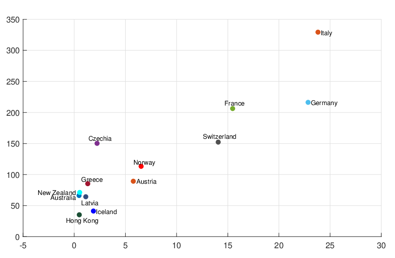
place yet. Figure 12, and 13 clearly demonstrate that the externally-exciting jump intensity ϱ
and the branching ratio after the government came into effect Ra are important factors that
determine the extinction time of the pandemic. In general, to reduce the extinction time of the
pandemic, the first priority for the authorities should be introducing restriction measures such as
national/subnational lockdown to reduce the intensity of the external imported cases, and
while the external imported cases are controlled and thereafter negligible, the governments
should simultaneously introduce enforced restrictions to prevent further transmission. If the
government intervention strategies were effectively implemented without a lack of civic spirit,
the infection rate of the virus after the these intervention measures come into place will be
reduced significantly, and therefore lead to a quicker elimination of the COVID-19 pandemic.
Note that the prediction for expected elimination time for regions and countries is based on
the assumption that the government intervention measures are still taking into place in some
form and propagation of the disease continues as in Phase 2. Relaxation of the government
intervention measures will inevitably delay the disease elimination for most regions and countries.
], respectively.
From Figure 11, we can see that for most countries and territories, the quicker the government
interventions come into effect, the faster the pandemic will end. However, some places like Hong
Kong and Iceland still have relatively fast elimination time even though it takes longer for
the government interventions to come into effect. This is probably because the restriction
measures for these places were imposed so early that reporting procedures were not properly in
place yet. Figure 12, and 13 clearly demonstrate that the externally-exciting jump intensity ϱ
and the branching ratio after the government came into effect Ra are important factors that
determine the extinction time of the pandemic. In general, to reduce the extinction time of the
pandemic, the first priority for the authorities should be introducing restriction measures such as
national/subnational lockdown to reduce the intensity of the external imported cases, and
while the external imported cases are controlled and thereafter negligible, the governments
should simultaneously introduce enforced restrictions to prevent further transmission. If the
government intervention strategies were effectively implemented without a lack of civic spirit,
the infection rate of the virus after the these intervention measures come into place will be
reduced significantly, and therefore lead to a quicker elimination of the COVID-19 pandemic.
Note that the prediction for expected elimination time for regions and countries is based on
the assumption that the government intervention measures are still taking into place in some
form and propagation of the disease continues as in Phase 2. Relaxation of the government
intervention measures will inevitably delay the disease elimination for most regions and countries.
Beside the conditional probability for the elimination time  , the epidemic size Nt given {
 ≤t} can
also be predicted according to the join expectation of Nt and {
≤t} can
also be predicted according to the join expectation of Nt and { ≤t} derived in Corollary 3.1. In Table
5, we report the 95% confidence interval for elimination time
≤t} derived in Corollary 3.1. In Table
5, we report the 95% confidence interval for elimination time  the condition expectation of
the elimination time
the condition expectation of
the elimination time  , E[
, E[ |
| ], the expected elimination date DateE, and the conditional
expectation of the epidemic size Nt, E[Nt|
], the expected elimination date DateE, and the conditional
expectation of the epidemic size Nt, E[Nt| ∩{
∩{ ≤t}] with t = E[
 |
| ], for regions
and countries with calibration parameters in Table 3. Note that, the regions and countries
with more confirmed COVID-19 cases before government interventions came into effect will
experience longer time to reach elimination state, like France, Germany, Italy, and New York.
And the corresponding expected epidemic size for these areas are also much larger. Note that
since we have smoothed the biggest jump of daily confirmed cases, adding up with the cases
which have been smoothed, the actual conditional expectation of the epidemic size is about
83113, which is very close to the current total confirmed cases 82,993 on 2020-05-27. In
general, not only the expected epidemic size is very close to the actual total confirmed cases for
the listed regions and countries, but also the estimated elimination date is very close to the
actual eradicate date. New Zealand is one typical example that can be used to demonstrate the
effectiveness of our model in predicting the key epidemiological quantities. New Zealand
authority has officially declared that the country has completely eradicated COVID-19 for
now with total of 1154 confirmed COVID-19 cases on 2020-06-08. This elimination date
and the final epidemic size are very close to what we predicted for New Zealand under the
two-phase dynamic contagion model, the predicted elimination date is around 2020-06-04 and the
predicted epidemic size is about 1250. More remarkably, the historical data we used for model
calibration for New Zealand is from 2020-03-12 to 2020-04-13, which is already one and
half months ago. This clearly shows that the two-phase dynamic contagion model is pretty
powerful in forecasting cumulative confirmed COVID-19 cases, predicting possible elimination
duration for the pandemic, and evaluating effectiveness of relevant government intervention
measures.
], for regions
and countries with calibration parameters in Table 3. Note that, the regions and countries
with more confirmed COVID-19 cases before government interventions came into effect will
experience longer time to reach elimination state, like France, Germany, Italy, and New York.
And the corresponding expected epidemic size for these areas are also much larger. Note that
since we have smoothed the biggest jump of daily confirmed cases, adding up with the cases
which have been smoothed, the actual conditional expectation of the epidemic size is about
83113, which is very close to the current total confirmed cases 82,993 on 2020-05-27. In
general, not only the expected epidemic size is very close to the actual total confirmed cases for
the listed regions and countries, but also the estimated elimination date is very close to the
actual eradicate date. New Zealand is one typical example that can be used to demonstrate the
effectiveness of our model in predicting the key epidemiological quantities. New Zealand
authority has officially declared that the country has completely eradicated COVID-19 for
now with total of 1154 confirmed COVID-19 cases on 2020-06-08. This elimination date
and the final epidemic size are very close to what we predicted for New Zealand under the
two-phase dynamic contagion model, the predicted elimination date is around 2020-06-04 and the
predicted epidemic size is about 1250. More remarkably, the historical data we used for model
calibration for New Zealand is from 2020-03-12 to 2020-04-13, which is already one and
half months ago. This clearly shows that the two-phase dynamic contagion model is pretty
powerful in forecasting cumulative confirmed COVID-19 cases, predicting possible elimination
duration for the pandemic, and evaluating effectiveness of relevant government intervention
measures.
Table 5: The 95% confidence interval for elimination time  , the conditional expectation of the
elimination time
, the conditional expectation of the
elimination time  , the expected elimination date and the conditional expectation of the epidemic
size Nt given
, the expected elimination date and the conditional expectation of the epidemic
size Nt given  ≤ t with t = E[
 |
| ] under the calibrated parameters (
 ,
, ,
, ,
, ,
, ) for these
regions and countries suggested in Table 3.
) for these
regions and countries suggested in Table 3.
_________________________________________________________________________________
|
|
|
|
|
 | ℙ( ∈(t1,t2)| ∈(t1,t2)|  ) = 95% ) = 95% | E[ | | ] ] | DateE | E[Nt| ∩{ ∩{ ≤t}] ≤t}] |
|
|
|
|
|
|
|
|
|
|
| Australia | (47,97) | 66 | 2020-05-30 | 7059.46 |
|
|
|
|
|
| Austria | (69,122) | 89 | 2020-06-21 | 15610.22 |
|
|
|
|
|
| China (Mainland) | (87,142) | 108 | 2020-05-22 | 69675.10 |
|
|
|
|
|
| Czechia | (111,216) | 150 | 2020-08-25 | 8932.448 |
|
|
|
|
|
| France | (166,272) | 206 | 2020-10-23 | 154112.00 |
|
|
|
|
|
| Germany | (175,285) | 216 | 2020-10-28 | 189116.50 |
|
|
|
|
|
| Greece | (59,127) | 85 | 2020-06-24 | 2650.07 |
|
|
|
|
|
| Hong Kong | (23,54) | 35 | 2020-05-05 | 945.81 |
|
|
|
|
|
| Iceland | (28,61) | 41 | 2020-05-11 | 1787.79 |
|
|
|
|
|
| Italy | (264,445) | 329 | 2021-02-13 | 276480.1 |
|
|
|
|
|
| Latvia | (40,102) | 64 | 2020-05-31 | 764.80 |
|
|
|
|
|
| New York | (149,261) | 192 | 2020-10-10 | 209311.80 |
|
|
|
|
|
| New Zealand | (49,107) | 71 | 2020-06-04 | 1249.77 |
|
|
|
|
|
| Norway | (83,162) | 113 | 2020-07-15 | 8024.73 |
|
|
|
|
|
| Switzerland | (121,203) | 152 | 2020-08-22 | 33414.19 |
|
|
|
|
|
| |
_________________________________________________________________________________
The conditional distribution of the final epidemic size N∞ can be obtained by numerically inverse the
probability generating function provided in Proposition 3.4. Since we assume the self-exciting jumps
follows an exponential distribution after government interventions came into effect, the final epidemic size
N∞ conditional on ℓ follows a mixed-Poisson distribution with probability mass function specified in
(3.16). Figure 14 demonstrates the conditional probability mass function of the difference between
the finial epidemic size N∞ and the total number of confirm cases Nℓ when government
interventions came into effect, i.e., ℙ , for some regions and countries under
the calibrated parameters (
, for some regions and countries under
the calibrated parameters ( ,
, ,
, ,
, ,
, ) for these regions and countries suggested in Table
3.
) for these regions and countries suggested in Table
3.
5 Concluding Remarks
In this paper, we have introduced a two-phase dynamic contagion process for modelling the current spread
of COVID-19. This model allows randomness to the infectivity of individuals rather than a constant
reproduction number as commonly assumed by standard models. Key episdemiological quantities, such as
the distribution of final epidemic size and expected epidemic duration, are derived and estimated based on
real data for various regions and countries. In addition, the associated time lag of the effect
of intervention in each country or region has been estimated, and our empirical results are
consistent to the incubation time of COVID-19 for most people found by existing medical study
such as Lauer et al. (2020). The aim of this paper is to demonstrate that our model, as a
representative of Hawkes-based processes, could be a valuable tool for epidemic modelling. In
fact, the vast literature of Hawkes-based processes would also be relevant and potentially be
applicable. For example, multivariate extensions of Hawkes-based processes, such as Embrechts
et al. (2011) for analysing financial high-frequency data, could be adopted for modelling the
cross-region epidemic contagion. Lévy-driven extensions, such as Qu et al. (2019) for portfolio
credit risk, may perform better in capturing the heavy tail property of epidemic distribution.
In addition, easing of the government interventions will lead to change of parameters and
delay extinction times. The model can be adjusted by introducing an additional phase with
change of parameters. When countries cycle between periods of restrictions and relaxations to
manage COVID-19, we can adjust the two-phase dynamic contagion model by replacing the
constant parameters to piecewise time dependent parameters. These are all proposed as future
research.
References
Acemoglu, D., Chernozhukov, V., Werning, I., and Whinston, M. D. (2020). A multi-risk SIR model
with optimally targeted lockdown. National Bureau of Economic Research Working Paper.
Aït-Sahalia, Y., Cacho-Diaz, J., and Laeven, R. J. (2015). Modeling financial contagion using mutually
exciting jump processes. Journal of Financial Economics, 117(3):585–606.
Allen, L. J. (2008). An introduction to stochastic epidemic models. In Allen, L. J., Brauer, F., Van den
Driessche, P., and Wu, J., editors, Mathematical Epidemiology, chapter 3, pages 81–130. Springer, Berlin.
Alvarez, F. E., Argente, D., and Lippi, F. (2020). A simple planning problem for COVID-19 lockdown.
National Bureau of Economic Research Working Paper.
Andersson, H. and Britton, T. (2000). Stochastic Epidemic Models and Their Statistical Analysis.
Springer, New York.
Atkeson, A. (2020). What will be the economic impact of COVID-19 in the US? rough estimates of
disease scenarios. National Bureau of Economic Research Working Paper.
Bacry, E., Delattre, S., Hoffmann, M., and Muzy, J.-F. (2013a). Modelling microstructure noise with
mutually exciting point processes. Quantitative Finance, 13(1):65–77.
Bacry, E., Delattre, S., Hoffmann, M., and Muzy, J.-F. (2013b). Some limit theorems for Hawkes
processes and application to financial statistics. Stochastic Processes and their Applications,
123(7):2475–2499.
Bailey, N. T. J. (1950). A simple stochastic epidemic. Biometrika, 37(3/4):193–202.
Bailey, N. T. J. (1953). The total size of a general stochastic epidemic. Biometrika, 40(1/2):177–185.
Bailey, N. T. J. (1957). The Mathematical Theory of Epidemics. Griffin, London.
Ball, F. (1983). The threshold behaviour of epidemic models. Journal of Applied Probability,
20(2):227–241.
Ball, F., Britton, T., and Neal, P. (2016). On expected durations of birth–death processes, with
applications to branching processes and SIS epidemics. Journal of Applied Probability, 53(1):203–215.
Ball, F. and Donnelly, P. (1995). Strong approximations for epidemic models. Stochastic Processes and
their Applications, 55(1):1–21.
Bartlett, M. (1949). Some evolutionary stochastic processes. Journal of the Royal Statistical Society.
Series B (Methodological), 11(2):211–229.
Bartlett, M. S. (1956). Deterministic and stochastic models for recurrent epidemics. In Proceedings of
the Third Berkeley Symposium on Mathematical Statistics and Probability, volume 4, pages 81–109.
Berger, D. W., Herkenhoff, K. F., and Mongey, S. (2020). An SEIR infectious disease model with
testing and conditional quarantine. National Bureau of Economic Research Working Paper.
Bowsher, C. G. (2007). Modelling security market events in continuous time: Intensity based,
multivariate point process models. Journal of Econometrics, 141(2):876–912.
Brauer, F., Van den Driessche, P., and Wu, J. (2008). Mathematical Epidemiology. Springer, Berlin.
Britton, T. (2010). Stochastic epidemic models: a survey. Mathematical Biosciences, 225(1):24–35.
Daley, D. J. and Gani, J. (1999). Epidemic Modelling: An Introduction. Cambridge University Press,
Cambridge.
Dassios, A. and Zhao, H. (2011). A dynamic contagion process. Advances in Applied Probability,
43(3):814–846.
Dassios, A. and Zhao, H. (2017a). Efficient simulation of clustering jumps with CIR intensity.
Operations Research, 65(6):1494–1515.
Dassios, A. and Zhao, H. (2017b). A generalised contagion process with an application to credit risk.
International Journal of Theoretical and Applied Finance, 20(1):1–33.
Diekmann, O., Heesterbeek, H., and Britton, T. (2013). Mathematical Tools for Understanding Infectious
Disease Dynamics. Princeton University Press, New Jersey.
Eichenbaum, M. S., Rebelo, S., and Trabandt, M. (2020). The macroeconomics of epidemics. National
Bureau of Economic Research Working Paper.
Embrechts, P., Liniger, T., and Lin, L. (2011). Multivariate Hawkes processes: an application to financial
data. Journal of Applied Probability, 48A:367–378.
Fuchs, C. (2013). Inference for Diffusion Processes: With Applications in Life Sciences. Springer-Verlag,
Berlin.
Guerrieri, V., Lorenzoni, G., Straub, L., and Werning, I. (2020). Macroeconomic implications of
COVID-19: Can negative supply shocks cause demand shortages? National Bureau of Economic Research
Working Paper.
Hawkes, A. G. (1971a). Point spectra of some mutually exciting point processes. Journal of the Royal
Statistical Society. Series B (Methodological), 33(3):438–443.
Hawkes, A. G. (1971b). Spectra of some self-exciting and mutually exciting point processes.
Biometrika, 58(1):83–90.
Keeling, M. J. and Rohani, P. (2008). Modeling Infectious Diseases in Humans and Animals. Princeton
University Press, New Jersey.
Kermack, W. O. and McKendrick, A. G. (1927). A contribution to the mathematical theory of
epidemics. Proceedings of the Royal Society, 115(772):700–721.
Large, J. (2007). Measuring the resiliency of an electronic limit order book. Journal of Financial
Markets, 10(1):1–25.
Lauer, S. A., Grantz, K. H., Bi, Q., Jones, F. K., Zheng, Q., Meredith, H. R., Azman, A. S., Reich,
N. G., and Lessler, J. (2020). The incubation period of coronavirus disease 2019 (COVID-19)
from publicly reported confirmed cases: estimation and application. Annals of Internal Medicine,
172(9):577–582.
Liu, Y., Gayle, A. A., Wilder-Smith, A., and Rocklöv, J. (2020). The reproductive number of COVID-19
is higher compared to SARS coronavirus. Journal of Travel Medicine, 27(2):1–4.
Martcheva, M. (2015). An Introduction to Mathematical Epidemiology. Springer, New York.
McKendrick, A. (1925). Applications of mathematics to medical problems. Proceedings of the
Edinburgh Mathematical Society, 44:98–130.
McNeill, W. H. (1976). Plagues and Peoples. Anchor, New York.
Qu, Y., Dassios, A., and Zhao, H. (2019). Efficient simulation of Lévy-driven point processes. Advances
in Applied Probability, 51(4):927–966.
Tian, H., Liu, Y., Li, Y., Wu, C.-H., Chen, B., Kraemer, M. U. G., Li, B., Cai, J., Xu, B., Yang, Q., Wang,
B., Yang, P., Cui, Y., Song, Y., Zheng, P., Wang, Q., Bjornstad, O. N., Yang, R., Grenfell, B. T., Pybus,
O. G., and Dye, C. (2020). An investigation of transmission control measures during the first 50 days of
the COVID-19 epidemic in China. Science, 368(6491):638–642.
![8> ϱμ 1 ϱμ 1
< --H-{κt≤-ℓ} + λs - -H-κ{t≤ℓ} e-κ(t-s), κ ⁄= 0,
E [λt|Fs] = > (3.5)
: λs + ϱ μH1 {t≤ℓ}(t- s), κ = 0,](Paper_Covid_19_DCP11x.png)
![8
>< ϱμH1{t≤-ℓ}(t-s) ϱμH1-{t≤ℓ} 1-e-κ(t-s)
E[N |F ] = Ns + κ + λs - κ κ , κ ⁄= 0, (3.6)
t s >: 1 2
Ns + λs(t- s)+ 2ϱμH 1{t≤ℓ}(t- s) , κ = 0,](Paper_Covid_19_DCP12x.png)
![8
>> - κ(t-s) λsμ2G- -κ(t-s)
>>> λsNse + λsμG + κ (t- s)e
< λ2s λsμ2G - κ(t-s) -2κ(t- s)
E[λtNt|Fs] = >> + -κ - --κ-- (e - e ), κ ⁄= 0, (3.8)
>>> 2 1 2
: λsNs + λs + λsμG (t - s)+ 2λsμ2G (t- s) , κ = 0](Paper_Covid_19_DCP16x.png)


 and the estimated
government interventions came into effect time for different regions and countries around the world.
The horizontal axis represents
and the estimated
government interventions came into effect time for different regions and countries around the world.
The horizontal axis represents  , and the vertical axis represents

 and the estimated
intensity for externally-exciting jumps for different regions and countries around the world. The
horizontal axis represents
and the estimated
intensity for externally-exciting jumps for different regions and countries around the world. The
horizontal axis represents  , and the vertical axis represents

 and the branching
ratio
and the branching
ratio 

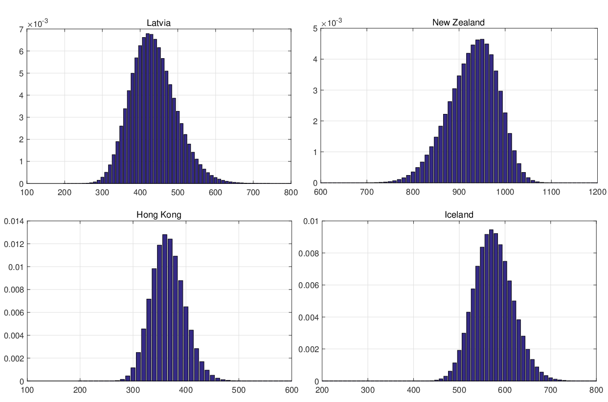
 for Latvia, New Zealand, Hong
Kong and Iceland under the calibrated parameters
for Latvia, New Zealand, Hong
Kong and Iceland under the calibrated parameters 


