Bivariate distributions

Activity 4.1   How would the scatter diagram change if the random variables were discrete rather than continuous?
$\blacksquare$

Answer 4.1   If the random variables are discrete, there will be a possibility of many points at the same place in the scatter diagram. For instance, if both $X$ and $Y$ take only positive integer values, we might get several observations with $X=1, Y=1$, leading to several points at $(1,1)$. The coincident points are hard to represent adequately in the scatter diagram. Sometimes a bigger dot is used when there are several points.
$\blacksquare$

Activity 4.2   Write down the marginal distribution of $Y$, and the conditional distributions of $X$ given $Y$.
$\blacksquare$

Answer 4.2   The marginal distribution of $Y$ is found from the column totals.

$$P(Y=0) = P[(X,Y)=(0,0)]+P[(X,Y)=(1,0)]+P[(X,Y)=(2,0)]$$

$$= 1/21+6/21+3/21 = 10/21.$$

$$P(Y=1) = P[(X,Y)=(0,1)]+P[(X,Y)=(1,1)]+P[(X,Y)=(2,1)]$$

$$= 4/21+6/21+0/21 = 10/21.$$

$$P(Y=2) = P[(X,Y)=(0,2)]+P[(X,Y)=(1,2)]+P[(X,Y)=(2,2)]$$

$$= 1/21+0/21+0/21 = 1/21.$$

The conditional distribution of $X$ for $Y=0$ is found by dividing the probabilities in the first column by the first column total.

$$P(X=0\vert Y=0) = P(X=0,Y=0)/P(Y=0)= (1/21)/(10/21) = 1/10,$$

$$P(X=1\vert Y=0) =P(X=1,Y=0)/P(Y=0)= (6/21)/(10/21) = 6/10=3/5,$$

$$P(X=2\vert Y=0) =P(X=2,Y=0)/P(Y=0)= (3/21)/(10/21) = 3/10.$$

The conditional distribution of $X$ for $Y=1$ is found by dividing the probabilities in the second column by the second column total.

$$P(X=0\vert Y=1) = P(X=0,Y=1)/P(Y=1)= (4/21)/(10/21) = 4/10=2/5,$$

$$P(X=1\vert Y=1) =P(X=1,Y=1)/P(Y=1)= (6/21)/(10/21) = 6/10=3/5,$$

$$P(X=2\vert Y=1) =P(X=2,Y=1)/P(Y=1)= (0/21)/(10/21) = 0.$$

The conditional distribution of $X$ for $Y=2$ is found by dividing the probabilities in the third column by the third column total. In fact, we know for sure that $X=0$ if $Y=2$.

$$P(X=0\vert Y=2) = P(X=0,Y=2)/P(Y=2)= (1/21)/(1/21) = 1,$$

$$P(X=1\vert Y=2) =P(X=1,Y=2)/P(Y=2)= (0/21)/(1/21) = 0,$$

$$P(X=2\vert Y=2) =P(X=2,Y=2)/P(Y=2)= (0/21)/(1/21) = 0.$$

$\blacksquare$

Activity 4.3   Nothing in principle stops us from thinking about the joint distribution of $(Y,Y)$, though this is a fairly pointless thing to do except for consistency of approach. From the last definition of $Y$, write down the table of probabilities for the joint distribution $(Y,Y)$.
$\blacksquare$

Answer 4.3  

Table 4.1: Probabilities for joint distribution of $(Y,Y)$

		$Y$
		0	$1$	$2$
	0	$10/21$	0	0
$Y$	$1$	0	$10/21$	0
	$2$	0	0	$1/21$

$\blacksquare$

Activity 4.4   Why isn't (4.1) any good for continuous variables?
$\blacksquare$

Answer 4.4   For continuous random variables $X,Y$, $P[X=x,Y=y]=0$ and $P[X=x]=0$, $P[Y=y]=0$. So for continuous variables, $P[X=x,Y=y]=P[X=x]P[Y=y]$ for all $x,y$ whether or not there is independence for $X$ and $Y$
$\blacksquare$

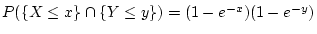
Activity 4.5   Show that if $P(\{X\le x \}\cap \{Y\le y\})=(1-e^{-x})(1-e^{-y})$ for all $x,y>0$, then $X$ and $Y$ are independent random variables, each with an exponential distribution. (Hint: use (4.2).)
$\blacksquare$

Answer 4.5   The righthand side of the result given is the product of the cdf for an exponential random variable $X$ with mean 1 and the cdf for an exponential random variable $Y$ with mean 1. So the result follows from (4.2).
$\blacksquare$

Activity 4.6   There are other ways to write the covariance. Show that

$$\operatorname{cov}(X, Y) = E[XY] -E[X]E[Y],$$

and

$$\operatorname{cov}(X, Y) = E[(X-E(X))Y] = E[X(Y-E(Y))].$$

$\blacksquare$

Answer 4.6  

$$\operatorname{cov}(X, Y) = E[(X-E(X))(Y-E(Y))]$$

$$=E[XY-XE(Y)-E(X)Y+E(X)E(Y)]$$

$$=E[XY]+E[-XE(Y)]+E[-E(X)Y]+E[E(X)E(Y)]$$

$$=E[XY]-E(Y)E[X]-E(X)E[Y]+E(X)E(Y)$$

$$=E[XY]-E(X)E(Y)$$

$$E[(X-E(X))Y] =E[XY-E(X)Y]$$

$$=E[XY]+E[-E(X)Y]$$

$$=E[XY]-E(X)E[Y]$$

$$=\operatorname{cov}(X,Y).$$

The remaining result follows by an argument symmetric with the last one.
$\blacksquare$

Activity 4.7   Suppose that $\operatorname{var}(X)=\operatorname{var}(Y)=1$, and that $X$ and $Y$ have correlation coefficient $\rho$. Show that it follows from $\operatorname{var}(X-\rho Y)\ge 0$ that $\rho^2\le 1$.
$\blacksquare$

Answer 4.7  

$$\le \operatorname{var}(X-\rho Y)$$ 0

$$=\operatorname{var}X -2\rho \operatorname{cov}(X,Y)+\rho^2\operatorname{var}Y$$

$$=1-2\rho^2 +\rho^2$$

$$=(1-\rho^2).$$

So $1-\rho^2\ge 0$, and so $\rho^2\le 1$.
$\blacksquare$